
Smart Readiness Metric
Disclaimer
On this page we are looking at how the Smart Readiness Metric is calculated in the publically available EPC Wrapper python reference code here:
Please be aware that the code we are looking at here (November 2026) should not be treated as a definitive representation of the final HEM/HEMIE methodology. This publicly available version is incomplete, remains under development and is subject to change. It should not be relied upon in any way.
The repository's README file makes this clear, stating:
“The EPC wrapper is currently in development and should not be used for any official purpose.”
The comments on this site are of the code at the time of anaylsis.
The comments on this site may be wrong.
Please use your own due diligence and look at the code yourself to confirm anything important.
How is the Smart Readiness metric calculated?
The epc_wrapper code runs the HEM calculation three times to compare annual electricity costs under three versions of the dwelling.
The scenarios are created in [smart_metric.py (line 158)].
Actual
This scenario starts from the dwelling as entered in the asessment, including whether it has an electricity smart meter and any energy technologies. A dwelling with a smart meter uses the Smart Metric tariff; one without uses the standard tariff. The wrapper standardises some items for this metric, including heating systems and hot-water provision, and applies the smart-meter implications based on the recorded meter status. It retains the dwelling’s heat batteries and handles its other batteries and electric vehicle according to the scenario rules. See [actual preprocessing (line 188)]( epc-wrapper/src/epc_wrapper/metrics/smart_metric.py:188).
Benchmark
This is a hypothetical smart-meter case. It uses standardised heating and hot-water arrangements, forces smart-meter presence, uses the smart meter tariff and adds benchmark assumptions for the presence of technologies including a home battery, solar PV, and an electric vehicle battery with vehicle-to-grid charging. See [benchmark preprocessing (line 215)].
Counterfactual
A hypothetical case without a smart meter, using the standard tariff. It also standardises heating and hot-water arrangements, removes home batteries and solar PV, adds a standard passive duct, and applies assumptions for an electric vehicle battery that cannot export to the grid. See [counterfactual preprocessing (line 238)](smart_metric.py:238) and [EV assumptions (line 1413)](smart_metric.py:1413).
The wrapper runs HEM once for each scenario, then calculates each scenario’s annual electricity cost from its energy imports and exports.
The tariff depends on the scenario’s smart-meter status; the metric calculation applies the import tariff to exports as well, and omits standing charges. See [cost calculation (line 472)](metrics.py:472) and [tariff setup (line 107)](smart_metric.py:107).
The three costs are then mapped to a score from 1 to 100. The benchmark cost currently marks a boundary point at 57.1 in the calculation formula:
- If the actual cost is at or below the benchmark cost, the score is between 57.1 and 100
- If the actual cost is above the benchmark, the counterfactual cost helps set a score between 1 and 57.1. See [score formula (line 542)] (metrics.py:542).
This is how the calculation is conducted:
Let:
- A = annual electricity cost in the actual scenario
- B = annual electricity cost in the benchmark scenario
- C = annual electricity cost in the counterfactual scenario
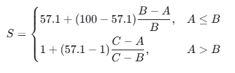
At or above the benchmark performance (A < B), the score runs from 57.1 when A=B, up to 100 when A=0.
Below the benchmark performance (A > B), the score runs from 57.1 at A=B, down to 1 at A=C.
Finally, the code clamps the result to the range 1–100. These equations are implemented in [`_smart_metric_boundary_score` (line 542)](metrics.py:542).
It would appear that a score of 100 would indicate the actual scenario’s calculated net electricity cost is zero or lower—that is, the value of exports offsets or exceeds the cost of imports under the tariff the code applies.
However, none of this information establishes what a future official EPC will say about the dwelling or what threshold would be required for a 'C' band rating. The boundary point could also be changed.
What electricity tariffs are used in the calculation?
The Smart Readiness metric uses electricity tariffs to put a cost on the energy imports and exports from each scenario.
At the time of analysis of the epc_wrapper code, the default “standard” and “smart” rates are both time series, but the standard rate is flat:
- Standard tariff: 25.16 p/kWh at every half-hour. It comes from the wrapper’s
metric_tariff_data.csvfile
- Default smart tariff : The default smart tariff in the supplied code is Octopus Intelligent Flux import pricing for eastern England, for January–December 2025. It varies every
half hour across 17,520 intervals ranging from 23.02 to 30.69 p/kWh, with an unweighted average of about 23.98 p/kWh. These figures are from the
Price_Inc_VATcolumn in the included file. The energy-cost result depends on when the dwelling imports or exports, not just on that average.
Mapping of the electricity tariff into each scenario depeneds on the presence of a smart meter as follows:
| Scenario | Tariff Used |
| Actual (with a smart meter) | Smart tariff |
| Actual (without a smart meter) | Standard tariff |
| Benchmark | Smart tariff |
| Counterfactual | Standard tariff |
Those defaults and scenario assignments are in [smart_metric.py (line 59)].
Old meter (no smart meter)
HEM simulates the home using the standard tariff, which is a flat 25.16 p/kWh in the code. After the simulation, the wrapper uses that same standard tariff to calculate the electricity cost.
Smart meter
HEM simulates the home using the Variable Time of Day Tariff column from the simulation tariff file (metric_tariff_data.csv). After the simulation, the
wrapper calculates the cost using the separate, half-hourly Intelligent Flux price profile. That data is stored in tariff_data_intelligent_flux_import_eastern_england_jan2025_to_dec2025.csv.
The Smart metric’s default configuration points to that file in [smart_metric.py (line 68)]. Flux prices range from about
23.02 to 30.69 p/kWh. The wrapper applies the price for each half-hour to both imports and exports.
The code allows the smart cost file and column to be overridden. See [tariff configuration (line 63)](smart_metric.py:63).
The cost calculation applies the chosen rate to electricity imports and uses the same rate for exports; exported energy is negative in the output, so it reduces the cost at that rate.
The code also leaves standing charge at zero for this metric. See [metrics.py (line 472)].
This all may change for the eventual official methodology.
The Benchmark scenario
Smart Meter
The benchmark scenario uses a smart meter.
Solar PV
The benchmark scenario includes solar PV. The kWp capacity of the solar PV is set to 60% of the ground floor area divided by 4.5. (roughly 1 kWp for every 7.5 m² of ground floor area). The assumed details are:
- Orientation: 180° from North, clockwise — ie: south-facing
- Pitch/tilt: 30°
- Base height: 10 m from the ground to the array’s lowest edge
- Shading: none
These are explicitly set in the benchmark PV setup in [smart_metric.py (line 800)].
The function comments that these are stubbed defaults, with other values taken from FHS notional logic.
If the dwelling already has PV panels, the benchmark code adjusts their peak power allocation but leaves their orientation and pitch as supplied.
It also explicitly adds or normalises a home battery, enables grid charging and export, and connects it to charge/discharge controls.
Home Battery
In the Benchmark scenario, the wrapper assumes a 9 kWh stationary home battery. If no home battery is present, it creates one with 80% round-trip efficiency, a maximum charge rate of 1.5 kW, and a maximum discharge rate of 1.25 kW. It is modelled indoors, allows grid charging, and is allowed to export to the grid. See [the benchmark battery setup (line 730)].
The code also gives it fixed monthly control thresholds:
- Charge threshold: 90%, with an import price threshold of 21.98 p/kWh
- Export threshold: 30%, with an export price threshold of 21.98 p/kWh
- Discharge threshold: 30%, with a discharge price threshold of 18.02 p/kWh
These are the control values supplied to HEM.
The battery can charge from the grid and export, so the scenario can model battery shifting across time.
The code also sets an existing home battery’s capacity to 9 kWh in the Benchmark scenario, while retaining its other physical properties. See [the battery control values (line 692)](smart_metric.py:692).
In contrast, the actual scenario uses the dwelling’s real battery details (if any), while the counterfactual removes home batteries.
 Print
